Create a Basic Contour Plot
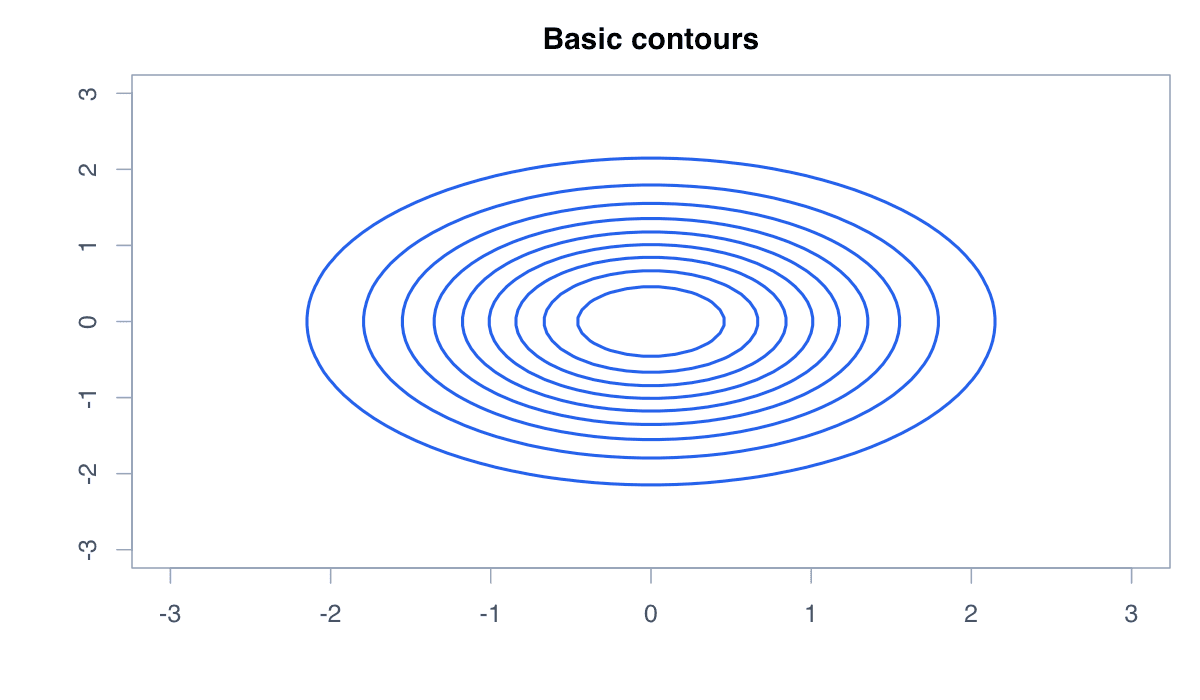
Contour lines connect combinations of x and y that share the same z value.
R Graphics · Contour Plot
Create basic, filled, labeled, custom-level, overlaid, and perspective-linked contours.
Contour plots connect locations with equal values on a two-dimensional surface. They translate three-dimensional structure into readable levels, gradients, peaks, and valleys.
Contour lines connect combinations of x and y that share the same z value.

Run the code, inspect how the visual encoding changes, and adapt the labels, scales, and styling to the analytical question rather than treating the defaults as fixed.
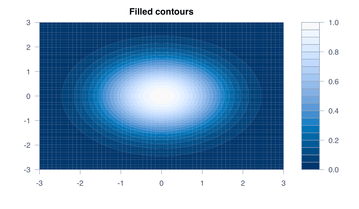
x<-seq(-3,3,length=60);y<-x;z<-outer(x,y,function(a,b) exp(-(a^2+b^2)/2));contour(x,y,z,col="#2563eb",lwd=2)Filled bands make ranges of surface height visually immediate.
Run the code, inspect how the visual encoding changes, and adapt the labels, scales, and styling to the analytical question rather than treating the defaults as fixed.
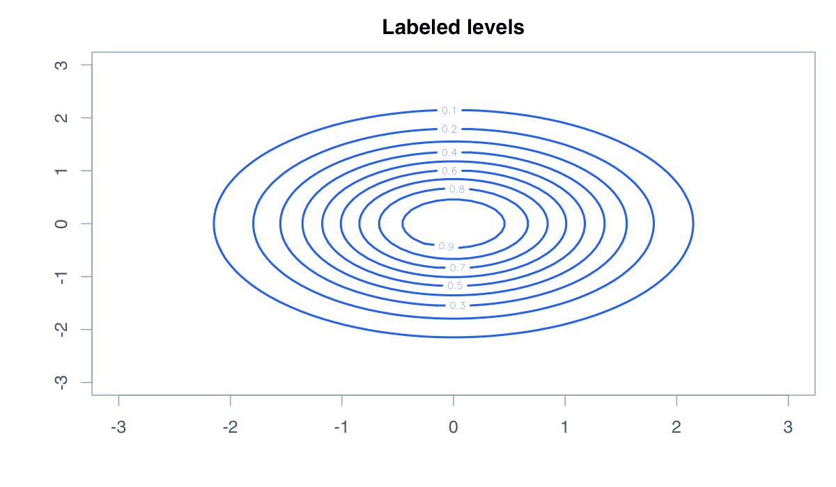
x<-seq(-3,3,length=60);y<-x;z<-outer(x,y,function(a,b) sin(a)*cos(b));filled.contour(x,y,z,color.palette=function(n) hcl.colors(n,"Blues 3"))Inline labels state the numeric value represented by each isoline.
Run the code, inspect how the visual encoding changes, and adapt the labels, scales, and styling to the analytical question rather than treating the defaults as fixed.
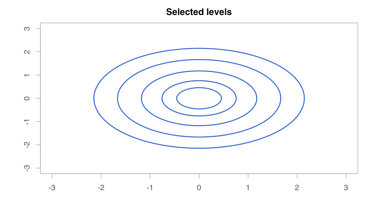
x<-seq(-3,3,length=60);y<-x;z<-outer(x,y,function(a,b) exp(-(a^2+b^2)/2));contour(x,y,z,drawlabels=TRUE,col="#2563eb")Custom levels focus attention on analytically important thresholds.
Run the code, inspect how the visual encoding changes, and adapt the labels, scales, and styling to the analytical question rather than treating the defaults as fixed.
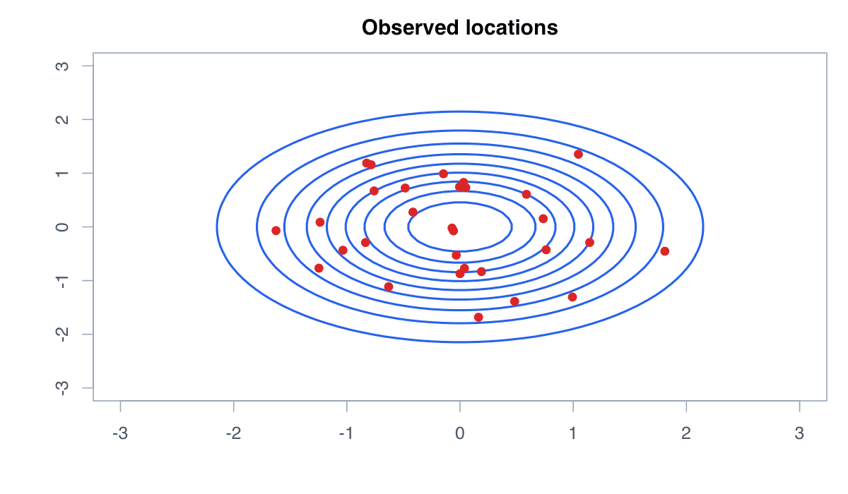
x<-seq(-3,3,length=60);y<-x;z<-outer(x,y,function(a,b) exp(-(a^2+b^2)/2));contour(x,y,z,levels=c(.1,.25,.5,.75,.9),lwd=2,col=hcl.colors(5,"Blues 3"))Points can show sampled locations on top of the interpolated or theoretical surface.
Run the code, inspect how the visual encoding changes, and adapt the labels, scales, and styling to the analytical question rather than treating the defaults as fixed.
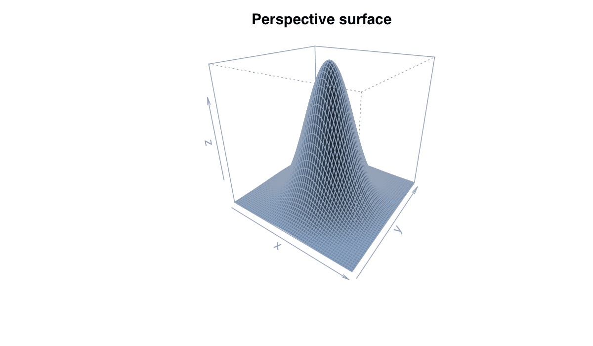
x<-seq(-3,3,length=60);y<-x;z<-outer(x,y,function(a,b) exp(-(a^2+b^2)/2));contour(x,y,z,col="#94a3b8");points(rnorm(30),rnorm(30),pch=19,col="#dc2626")A perspective plot provides a complementary three-dimensional view of the same matrix.
Run the code, inspect how the visual encoding changes, and adapt the labels, scales, and styling to the analytical question rather than treating the defaults as fixed.
x<-seq(-3,3,length=40);y<-x;z<-outer(x,y,function(a,b) exp(-(a^2+b^2)/2));persp(x,y,z,theta=35,phi=25,col="#93c5fd",shade=.4,xlab="X",ylab="Y",zlab="Z")