Draw a Basic Polygon
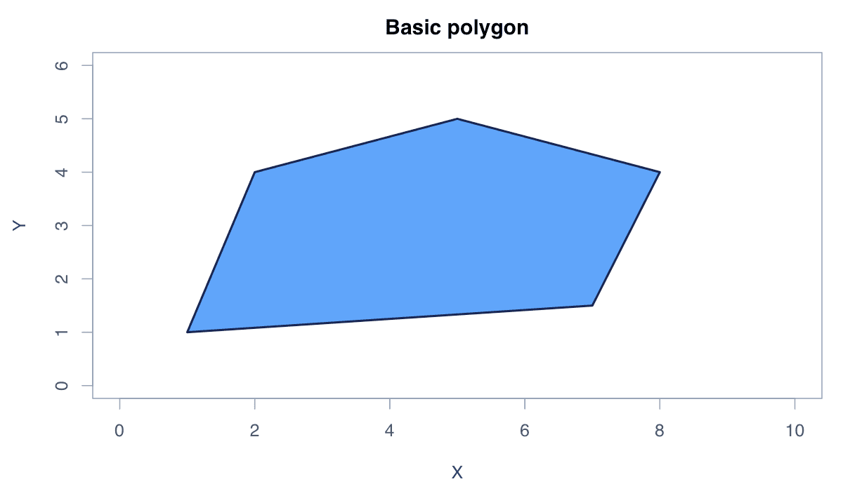
A polygon connects coordinate pairs and closes the final edge automatically.
R Graphics · Polygon Plot
Learn closed shapes, transparent overlays, areas under curves, confidence bands, highlighted regions, and layered polygons.
polygon() joins ordered coordinates into a closed shape. It is a versatile low-level tool for filled regions, uncertainty bands, map-like shapes, and emphasis within an existing plot.
A polygon connects coordinate pairs and closes the final edge automatically.

Provide x and y vectors in boundary order. Fill and border colors define the interior and outline.
plot(1, type = "n", xlim = c(0, 5), ylim = c(0, 5), xlab = "X", ylab = "Y")
polygon(c(1, 4, 3.5, 2, .7), c(1, 1.2, 4, 4.5, 3),
col = "#60a5fa", border = "#172554", lwd = 2)Transparency allows overlapping regions to remain visible.
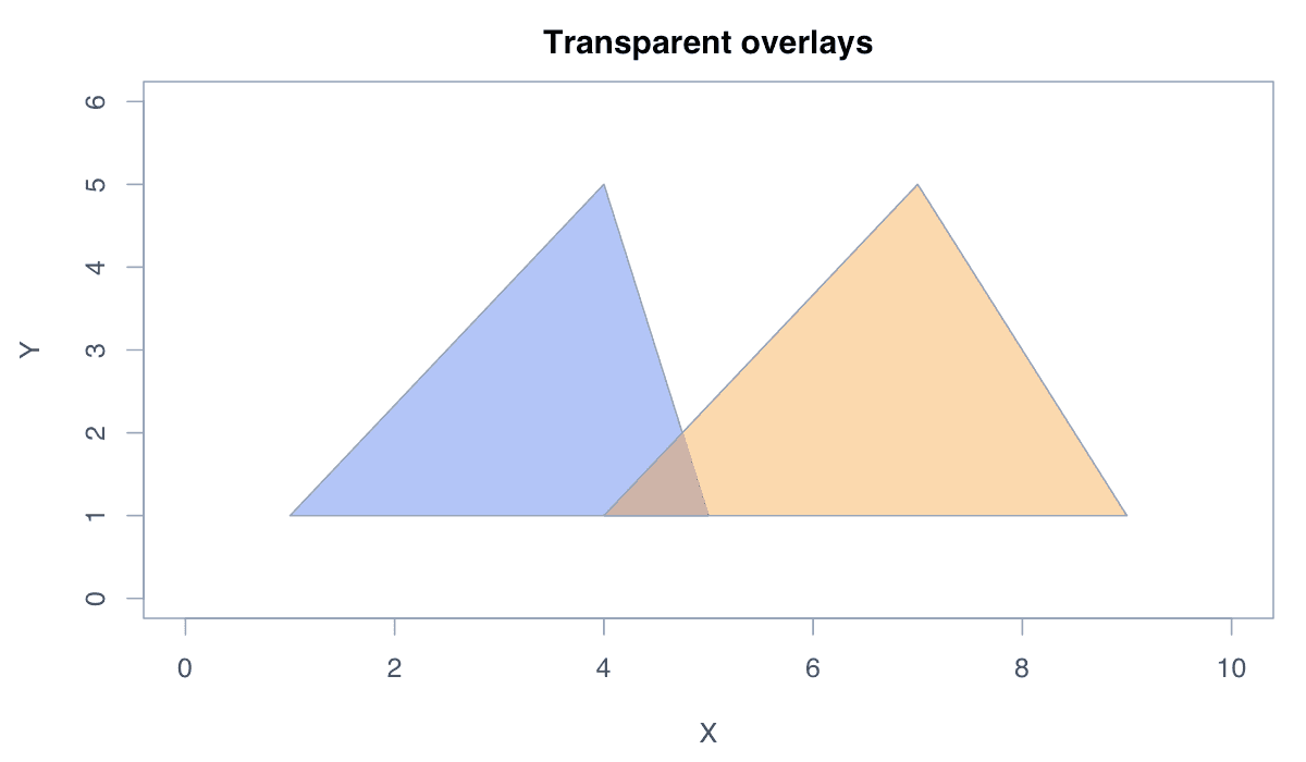
adjustcolor() adds alpha transparency, making intersections legible without requiring a separate pattern.
plot(1, type = "n", xlim = c(0, 7), ylim = c(0, 5), axes = FALSE, xlab = "", ylab = "")
polygon(c(1,4,3,1), c(1,1,4,1), col = adjustcolor("#2563eb",.45), border = "#2563eb")
polygon(c(3,6,5,3), c(1,1,4,1), col = adjustcolor("#f59e0b",.45), border = "#f59e0b")A filled polygon can emphasize accumulated area beneath a line.
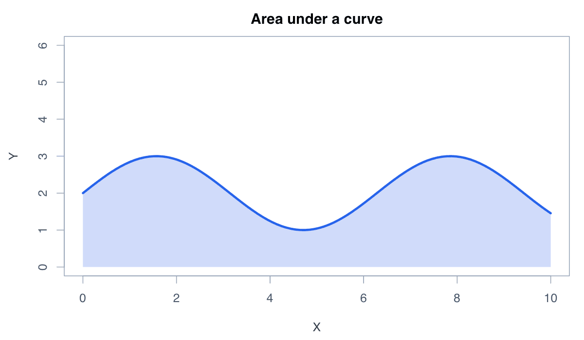
Combine the curve coordinates with baseline endpoints so the polygon closes along the axis.
x <- seq(0, 2*pi, length.out = 150); y <- sin(x) + 1
plot(x, y, type = "n", xlab = "x", ylab = "sin(x) + 1")
polygon(c(x, rev(x)), c(y, rep(0, length(y))), col = "#dbeafe", border = NA)
lines(x, y, col = "#2563eb", lwd = 3)Two boundaries can be joined into one polygon representing uncertainty.
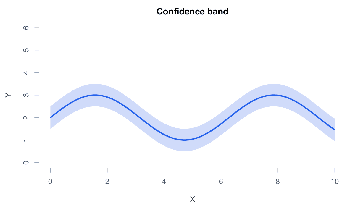
Append the upper boundary to the reversed lower boundary so the shape does not cross itself.
x <- 1:30; fit <- 2 + .2*x; se <- .5 + x/100
plot(x, fit, type = "n", ylim = range(fit-se, fit+se))
polygon(c(x, rev(x)), c(fit-se, rev(fit+se)), col = adjustcolor("#2563eb",.2), border = NA)
lines(x, fit, col = "#2563eb", lwd = 3)A rectangle-shaped polygon can mark a meaningful interval behind the data.
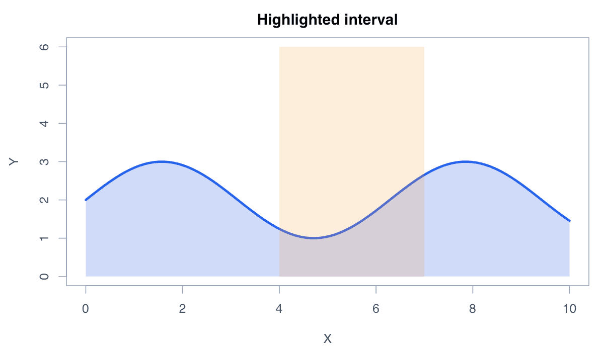
Draw the highlighted region before the series and use transparency so gridlines and values remain readable.
x <- 1:20; y <- cumsum(rnorm(20))
plot(x, y, type = "n")
polygon(c(8, 13, 13, 8), c(par("usr")[3], par("usr")[3], par("usr")[4], par("usr")[4]),
col = adjustcolor("#f59e0b",.2), border = NA)
lines(x, y, col = "#172554", lwd = 2)Multiple polygons can form a richer analytical or illustrative graphic.
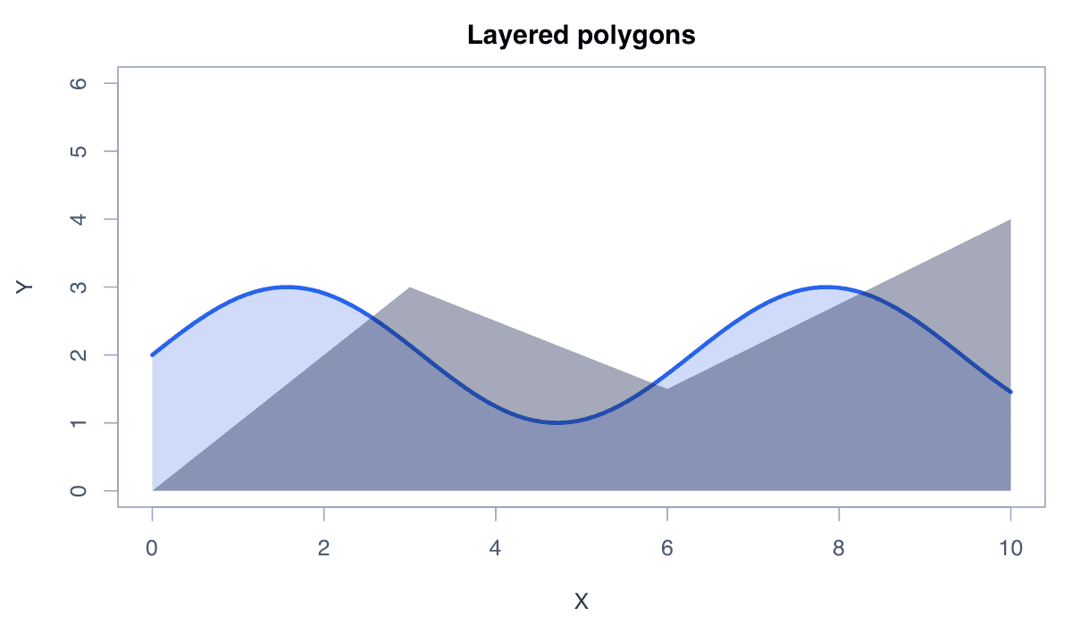
Control the drawing order: background shapes first, then foreground shapes, outlines, and annotations.
plot(1, type = "n", xlim = c(0, 10), ylim = c(0, 6), axes = FALSE, xlab = "", ylab = "")
polygon(c(0,3,5,7,10,10,0), c(1,4,2.5,5,2,0,0), col = "#dbeafe", border = NA)
polygon(c(0,3,5,7,10,10,0), c(.5,2.5,1.5,3,1,0,0), col = "#2563eb", border = NA)