R Graphics · Radar Chart

Comparing Multivariate Profiles with Radar Charts in R

Build single, multiple, normalized, filled, labeled, and package-based radar profiles.

6 examplesReproducible R code

Before you begin

Choose the variation that serves the analysis

Radar charts place variables on radial axes and join their values into profiles. They are useful for a few similarly scaled indicators, but exact comparisons are often clearer in parallel-coordinate or dot plots.

Examples: 06
Levels: Beginner + Intermediate

Example 01Base RBeginner

Create a Basic Radar Profile

A radar profile joins values positioned on equally spaced radial axes.

R-generated example output.

Run the code, inspect how the visual encoding changes, and adapt the labels, scales, and styling to the analytical question rather than treating the defaults as fixed.

RRun this code

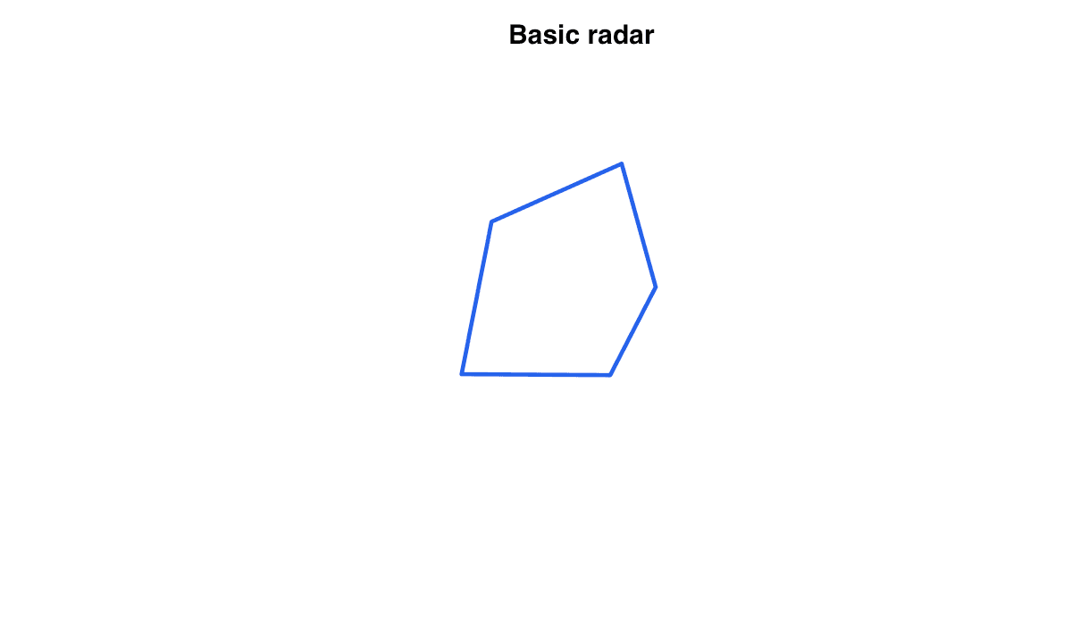
v<-c(4,7,6,8,5);ang<-seq(0,2*pi,length.out=6);r<-c(v,v[1]);plot(cos(ang)*r,sin(ang)*r,type="l",asp=1,lwd=3,col="#2563eb",axes=FALSE,xlab="",ylab="")

Example 02Base RBeginner

Fill the Radar Polygon

A translucent fill emphasizes the overall profile while preserving the grid beneath it.

Run the code, inspect how the visual encoding changes, and adapt the labels, scales, and styling to the analytical question rather than treating the defaults as fixed.

RRun this code

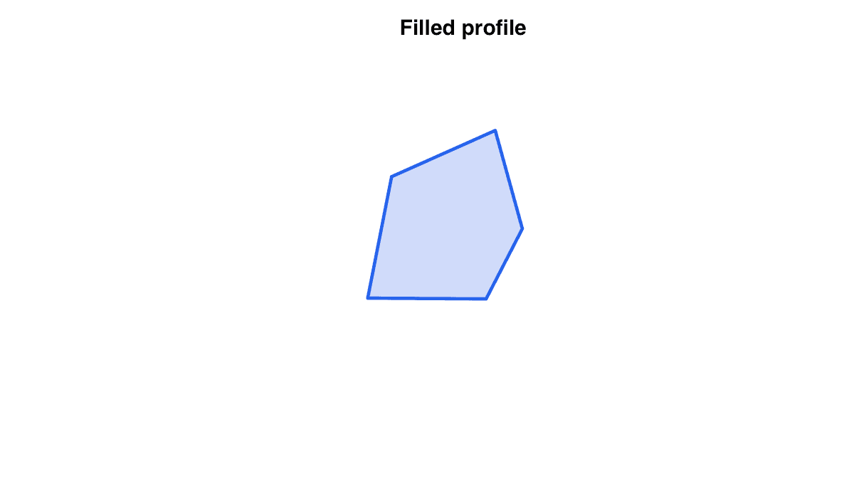
v<-c(4,7,6,8,5);ang<-seq(0,2*pi,length.out=6);r<-c(v,v[1]);plot(cos(ang)*10,sin(ang)*10,type="n",asp=1,axes=FALSE,xlab="",ylab="");polygon(cos(ang)*r,sin(ang)*r,col=adjustcolor("#2563eb",.25),border="#2563eb",lwd=3)

Example 03Base RBeginner

Add a Radial Reference Grid

Concentric reference polygons help readers judge values along each spoke.

Run the code, inspect how the visual encoding changes, and adapt the labels, scales, and styling to the analytical question rather than treating the defaults as fixed.

RRun this code

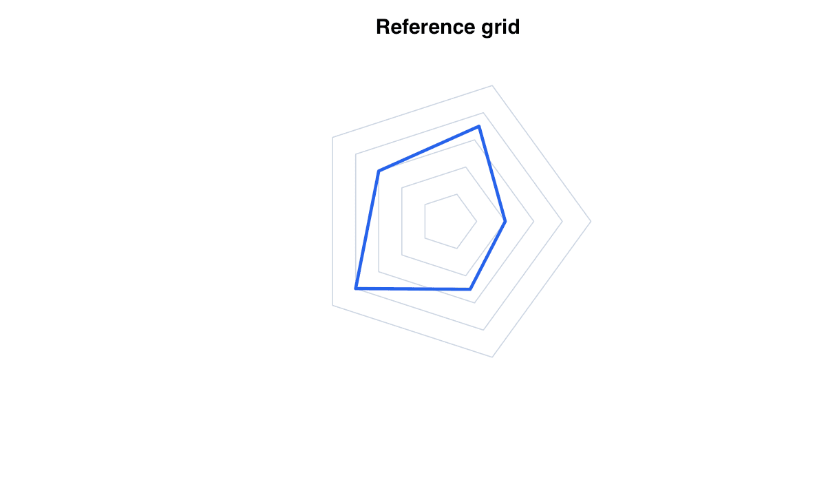
n<-5;ang<-seq(0,2*pi,length.out=n+1);plot(c(-10,10),c(-10,10),type="n",asp=1,axes=FALSE,xlab="",ylab="");for(k in c(2,4,6,8,10))polygon(cos(ang)*k,sin(ang)*k,border="#cbd5e1");segments(0,0,cos(ang[-6])*10,sin(ang[-6])*10,col="#cbd5e1")

Example 04Base RIntermediate

Compare Two Profiles

Multiple outlined profiles reveal contrasting strengths across a small set of indicators.

Run the code, inspect how the visual encoding changes, and adapt the labels, scales, and styling to the analytical question rather than treating the defaults as fixed.

RRun this code

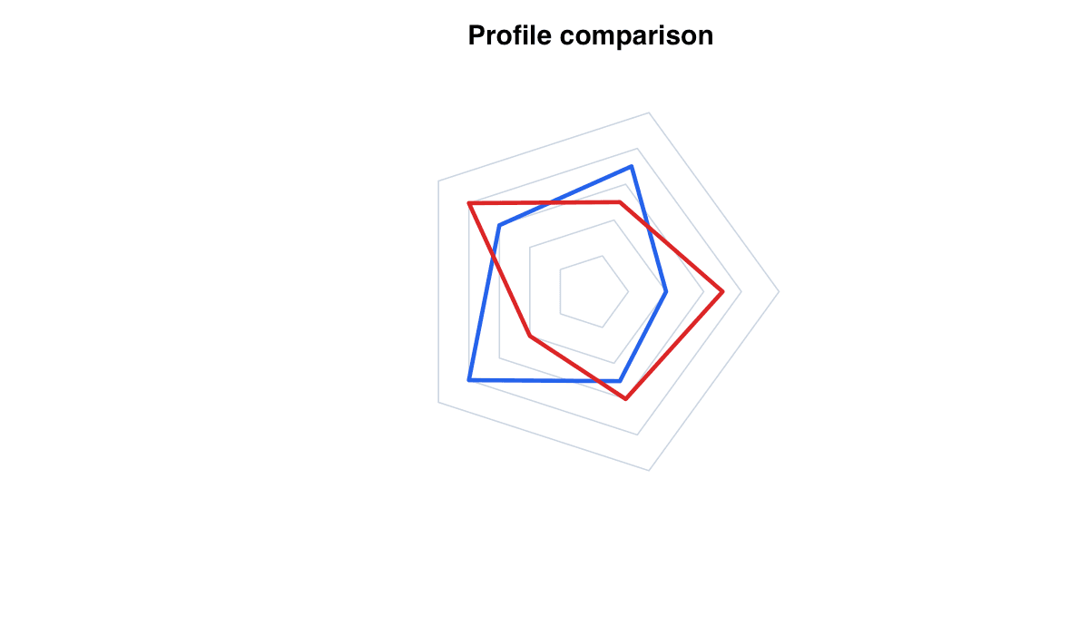
a<-c(4,7,6,8,5);b<-c(7,5,8,4,6);ang<-seq(0,2*pi,length.out=6);plot(c(-10,10),c(-10,10),type="n",asp=1,axes=FALSE,xlab="",ylab="");polygon(cos(ang)*c(a,a[1]),sin(ang)*c(a,a[1]),border="#2563eb",lwd=3);polygon(cos(ang)*c(b,b[1]),sin(ang)*c(b,b[1]),border="#dc2626",lwd=3)

Example 05Base RIntermediate

Label Every Indicator

Labels around the perimeter identify the meaning of each radial axis.

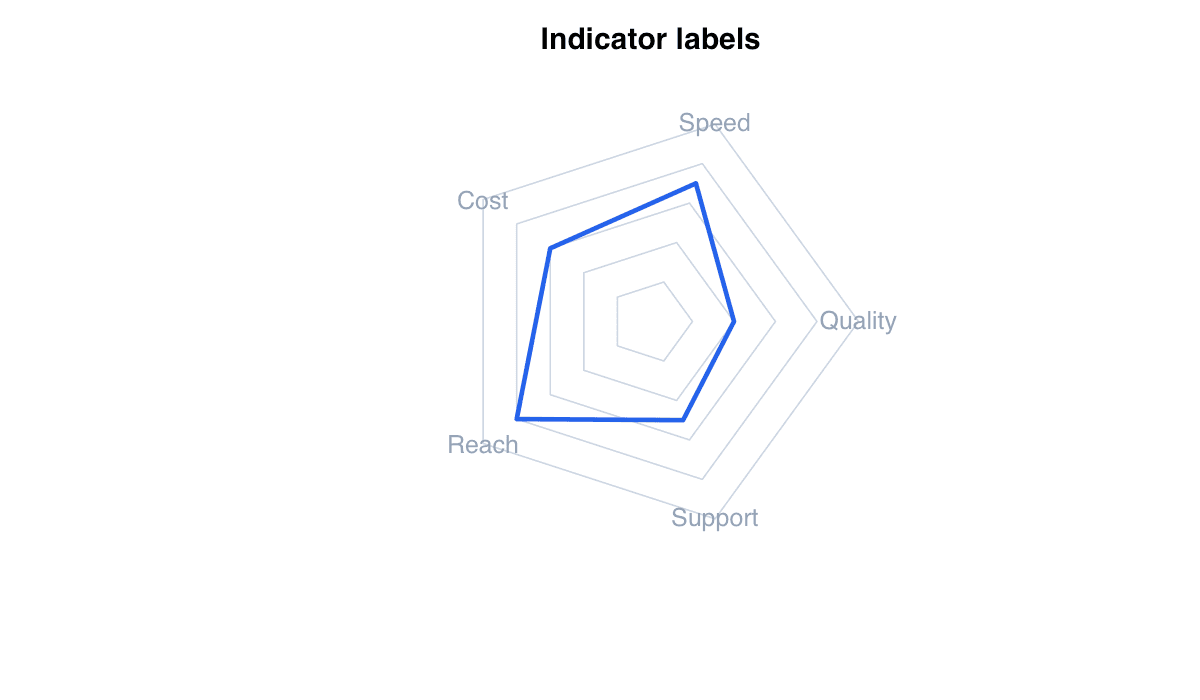
Run the code, inspect how the visual encoding changes, and adapt the labels, scales, and styling to the analytical question rather than treating the defaults as fixed.

RRun this code

labs<-c("Quality","Speed","Cost","Reach","Support");v<-c(4,7,6,8,5);ang<-seq(0,2*pi,length.out=6);plot(c(-11,11),c(-11,11),type="n",asp=1,axes=FALSE,xlab="",ylab="");polygon(cos(ang)*c(v,v[1]),sin(ang)*c(v,v[1]),border="#2563eb",lwd=3);text(cos(ang[-6])*10,sin(ang[-6])*10,labs)

Example 06Base RIntermediate

Normalize Indicators Before Comparing

Normalization places differently scaled indicators on a common radial range.

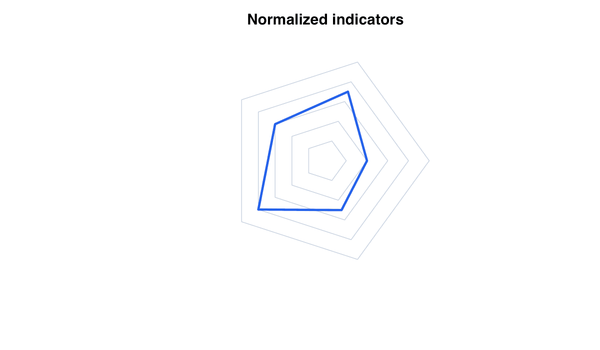
Run the code, inspect how the visual encoding changes, and adapt the labels, scales, and styling to the analytical question rather than treating the defaults as fixed.

RRun this code

raw<-c(quality=82,speed=14,cost=240,reach=60,support=4.5);mins<-c(0,0,0,0,0);maxs<-c(100,20,500,100,5);scaled<-(raw-mins)/(maxs-mins)*10;scaled